Decimals of accuracy: choosing a number system by its precision profile

Every number system spends its bits on two things: range (how large and how small a value it can hold) and precision (how finely it divides the values in between). A precision profile shows where each system puts them. It plots, at every magnitude, how many decimal digits the system keeps.

This tutorial uses the profile to compare five 16-bit number systems. It then zooms into the magnitudes a signal-processing pipeline actually uses, notices that the standard b-posit wastes most of its encodings outside them, and fits a b-posit to the job.

The measure

For an encoding x whose next larger encoding is x+, the spacing is ulp(x) = x+ - x. Rounding a real number to the nearest encoding makes a relative error of at most ulp / (2|x|). Expressed in decimal digits, that is Gustafson’s decimals of accuracy (The End of Error, 2015):

decimals(x) = -log10( ulp(x) / (2 |x|) )

A system has 0 decimals at magnitudes it cannot represent, below its smallest positive value or above its largest. (Averaged over an ulp, the relative error is ulp / (4|x|): the same curve, shifted up by log10(2) = 0.30.)

The profiles come from precision_profile_of<T>() in universal/utility/precision_profile.hpp. For types of up to 16 bits it decodes every encoding, so each curve below has about 32,000 points. Wider types are sampled a few points per binade.

Generating the data

Build the comparison application. Run it with a directory, and it writes one CSV file per number system there, alongside the tables quoted below:

cmake -S . -B build -DUNIVERSAL_BUILD_APPLICATIONS=ON
cmake --build build --target dsp_precision_profiles
mkdir -p profiles
build/applications/mixed-precision/dsp/dsp_precision_profiles profiles

The figures are drawn by tools/notebooks/plot_precision_profiles.py, which needs matplotlib.

The full range

First, the whole picture: five 16-bit systems across everything they can represent.

python3 tools/notebooks/plot_precision_profiles.py \
    profiles/int16.csv profiles/Q15.csv profiles/fp16.csv profiles/lns_16_10_.csv profiles/bposit_16_6_5_.csv \
    --title "16-bit number systems: decimals of accuracy across the full range" \
    -o 16bit-full-range.png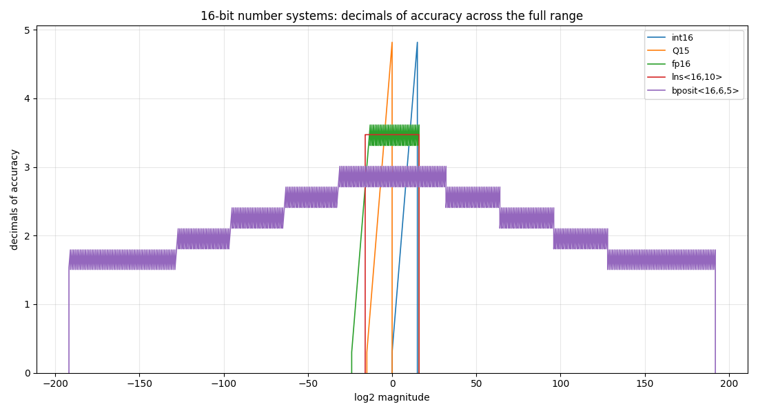

Each system’s shape is its design:

• int16 starts at 1, its smallest positive value, and gains precision with magnitude: the spacing is always 1, so a larger value is relatively more precise. It peaks at 4.8 decimals at 2^15.
• Q15, fixpnt<16,15>, is the same line shifted down by 15 binades. It covers 2^-15 to just below 1.
• fp16, cfloat<16,5>, has a flat top: 10 fraction bits, 3.3 to 3.6 decimals, in every binade from 2^-14 to 2^15. Below that, its subnormals ramp down to 2^-24.
• lns<16,10> is perfectly flat at 3.47 decimals. A logarithmic system’s relative spacing is the same everywhere, here across 2^-16 to 2^16.
• bposit<16,6,5>, the standard bounded posit, is a tent. It keeps 2.7 to 3.0 decimals near 1 and steps down by one fraction bit every 32 binades, out to 2^+-192. Its regime is capped, so it never drops below 4 fraction bits (1.5 decimals) and stops sharply at its bounded range.

The picture shows the trade every 16-bit format makes. The b-posit spans 384 binades and the integer formats about 15. The formats with the widest range keep the fewest digits.

Zooming into the region of interest

A digital signal processing (DSP) pipeline does not use 384 binades:

• The signal band. Samples are normalized to [-1, 1). The precision just below 1.0 sets the quantization noise floor, at about 6.02 dB of SQNR per bit.
• The floor. Small filter coefficients and the tail of a spectrum sit down to about 2^-15 (-90 dBFS).
• FFT growth. An N-point FFT grows magnitudes by up to log2(N) bits: 2^8, 2^10 and 2^12 for N = 256, 1024 and 4096.

So the region of interest is [2^-15, 2^12]. The same five curves, restricted to it with --xmin and --xmax. --dsp shades the signal band, marks the FFT growth and adds an SQNR axis:

python3 tools/notebooks/plot_precision_profiles.py \
    profiles/int16.csv profiles/Q15.csv profiles/fp16.csv profiles/lns_16_10_.csv profiles/bposit_16_6_5_.csv \
    --dsp --xmin -32 --xmax 24 \
    --title "16-bit number systems: the region of interest" \
    -o 16bit-region-of-interest.png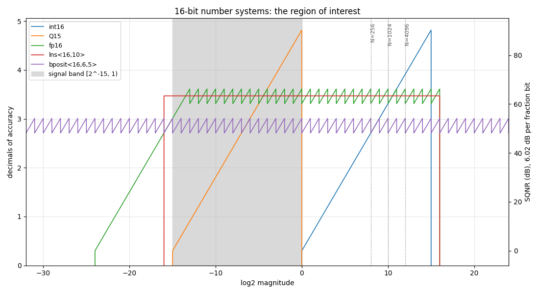

At this scale each binade’s sawtooth is visible. Precision is best at the top of a binade and drops by log10(2) where the spacing doubles. In this region:

• Q15 is the most precise in the signal band, 4.52 decimals in [0.5, 1). It has nothing above 1.0, so an FFT must rescale at every stage. Below the band it falls off a cliff: at 2^-15 it is down to its last bit.
• int16 cannot hold the signal band at all without a scale factor.
• fp16 holds 3.3 to 3.6 decimals across the region, except its lowest binade: 2^-15 is subnormal, at 3.0. lns<16,10> is flat at 3.47.
• bposit<16,6,5> holds 2.7 to 3.0, the least of the floating-point formats. Its range reaches some 180 binades beyond the region on each side, and it pays for that range here.

The standard b-posit’s range is wasted

A 16-bit format has 32,767 positive encodings. How many of them land in the region of interest?

type	range (log2)	positive encodings in [2^-15, 2^12]
bposit<16,6,5>	-192 .. 192	21.1 %
fp16	-24 .. 16	85.5 %
lns<16,10>	-16 .. 16	84.4 %

Nearly four in five of the standard b-posit’s encodings represent magnitudes between 2^-192 and 2^-15, or between 2^12 and 2^192. A DSP pipeline never produces them. Those encodings are not free. Every bit the regime spends reaching them is a fraction bit that the values in the region do not get.

Fitting the range

A b-posit’s range is set by its maximum regime size rS and its exponent size eS: it spans 2^+-(rS 2^eS). The question is which configuration covers [2^-15, 2^12] with the fewest bits spent on range. The application prints the candidates:

type	range (log2)	encodings in the region	decimals in [0.5, 1)	worst in the region	floor (bits)
bposit<16,6,5>	-192 .. 192	21.1 %	2.71	2.71	4
bposit<16,6,3>	-48 .. 48	67.2 %	3.31	3.01	6
bposit<16,6,2>	-24 .. 24	89.8 %	3.61	2.71	7
bposit<16,5,2>	-20 .. 20	89.8 %	3.61	2.71	8
bposit<16,4,2>	-16 .. 16	92.2 %	3.61	3.01	9
bposit<16,3,1>	-6 .. 6	100.0 %	3.91	0.00	11

• bposit<16,4,2> is the best fit. Its range, 2^+-16, just covers the region. It puts 92% of its encodings there and keeps at least 3.01 decimals across all of it. It never drops below 9 fraction bits, against 4 for the standard configuration.
• bposit<16,5,2> buys four more binades of headroom, up to 2^20 (million-point FFTs), for one bit of floor. It is the choice if the growth budget is uncertain.
• bposit<16,3,1> shows the limit. All its encodings fall inside the region, but its 2^+-6 range does not cover it: 0 decimals at 2^-15 and at 2^10. A fit must cover the region, not just sit inside it.

The fitted b-posits against fp16, the standard b-posit and Q15:

python3 tools/notebooks/plot_precision_profiles.py \
    profiles/Q15.csv profiles/fp16.csv profiles/bposit_16_6_5_.csv profiles/bposit_16_5_2_.csv profiles/bposit_16_4_2_.csv \
    --dsp --xmin -32 --xmax 24 \
    --title "Fitting the b-posit range to the region of interest" \
    -o 16bit-bposit-fit.png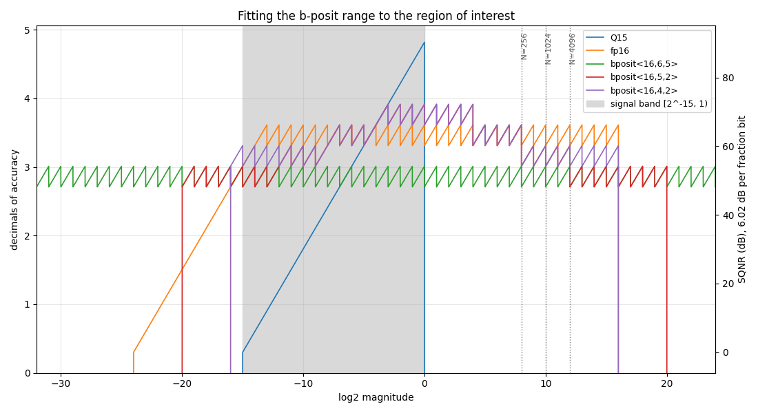

The two fitted b-posits coincide from 2^-12 to 2^12, peaking at 3.91 decimals. They part only at the edges of the region, where bposit<16,4,2> keeps one more bit.

• Against the standard bposit<16,6,5>, the fitted configurations are one to three bits ahead at every magnitude in the region: up to 0.9 decimals, or 18 dB of SQNR, near 1.0.

• Against fp16 the comparison is local, because a b-posit’s precision is tapered:

  magnitudes	bposit<16,4,2> against fp16
  2^-4 to 2^4	one bit ahead: 3.61 to 3.91 decimals against 3.31 to 3.61
  2^-8 to 2^-4, and 2^4 to 2^8	the same
  2^-15 to 2^-8, and 2^8 to 2^12	one bit behind (tied at 2^-15, where fp16 is subnormal)

  The b-posit concentrates its bits around 1.0, where a normalized signal’s large samples, and most of its power, live. fp16 spreads them evenly.

That is the paper’s point (Closing the Gap Between Float and Posit Hardware Efficiency, arXiv 2603.01615): a b-posit with a smaller eS suffices for signal processing, and the range it gives up is range the workload never uses.

The same at 32 bits

The region of interest does not change with the width, so the same configuration fits:

python3 tools/notebooks/plot_precision_profiles.py \
    profiles/Q31.csv profiles/float.csv profiles/bposit_32_6_5_.csv profiles/bposit_32_4_2_.csv \
    --dsp --xmin -40 --xmax 24 \
    --title "32-bit: the same fit" \
    -o 32bit-bposit-fit.png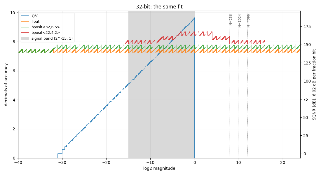

type	range (log2)	decimals in [0.5, 1)	worst in the region	floor (bits)
float	-149 .. 128	7.22	7.22	0 (subnormals)
bposit<32,6,5>	-192 .. 192	7.53	7.53	20
bposit<32,5,2>	-20 .. 20	8.43	7.53	24
bposit<32,4,2>	-16 .. 16	8.43	7.83	25

bposit<32,4,2> beats float across the whole region, by 0.6 to 1.2 decimals (2 to 4 bits), and never drops below 25 fraction bits. Q31 is more precise in the signal band, but like Q15 it has no headroom and fades below it.

Summary

• Start with the full range. The profile’s shape shows how a system divides its bits between range and precision.
• Then zoom in. Restrict the plot to the magnitudes the computation actually produces: the region of interest.
• Count where the encodings land. Encodings outside the region are not just unused; the bits that reach them come out of the precision inside it.
• Size the format to the region. For a b-posit, choose rS and eS so that 2^+-(rS 2^eS) just covers the region. Here bposit<16,4,2> is one to three bits ahead of the standard bposit<16,6,5> everywhere in the region, and one bit ahead of fp16 around 1.0.

The DSP results are also summarized in the bposit page, and the application that computes them is applications/mixed-precision/dsp/precision_profiles.cpp.