Givens and Householder in pictures
Four animations show what a Givens rotation and a Householder reflector do, how each one builds a QR factorization, how rotations drive the QR iteration for singular values, and what happens to orthogonality when a rotation is computed in a narrow number format. The history and references behind them are in givens-householder-history.md. The interactive explorer lets you drag a column through a rotation or reflector computed in a narrow format, together with a second column carried along by the same operator. This page is part of the series in #666.
The figures are generated by tools/givens_householder_svg.py, which uses
only the Python standard library:
python3 tools/givens_householder_svg.py # writes docs/img/gh-*.svgThe animations are SVG’s own SMIL elements, with no script, so they play in
any browser, including through an <img> tag. Rerunning the script
reproduces the committed files byte for byte.
1. Two ways to put a vector on an axis
Section titled “1. Two ways to put a vector on an axis”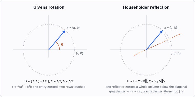
Both operators take to with , and both are orthogonal, so neither changes a length.
- The rotation turns through its own angle . Its matrix needs only and ; the angle itself is never computed. .
- The reflection flips across a mirror. The mirror is the line perpendicular to , which bisects the angle between and the axis. with , and . For , computing directly cancels when is small, so the first component is computed as (Parlett’s form). If and , is already on the axis, , and the identity is used in place of a reflector.
In two dimensions the two do the same job. The difference shows in dimensions. A rotation acts on two coordinates and zeroes one of them. A reflector acts on all of them and zeroes every coordinate but the first in a single step. That difference decides which one each algorithm below uses.
The figure reflects onto , the sign MTL5’s householder() uses for
a vector with (Parlett’s form). LAPACK’s dlarfg reflects the same
vector onto , across the other bisector. Both choices avoid
cancellation; householder-reflector-forms.md
compares them.
2. QR one entry at a time, or one column at a time
Section titled “2. QR one entry at a time, or one column at a time”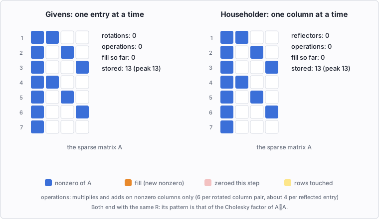
The same sparse matrix is triangularized twice. On the left, each rotation turns one row below the diagonal into the pivot row and zeroes one entry. On the right, each reflector zeroes a whole column below the diagonal. The yellow band marks the rows each step touches. Orange cells are fill: entries that were zero in and become nonzero.
| Givens | Householder | |
|---|---|---|
| steps | 18 rotations | 4 reflectors |
| operations (sparse-aware count) | 282 | 218 |
| fill created | 15 | 15 |
| peak entries stored | 21 | 28 |
The counts come from the script’s symbolic run. They count multiplies and adds on the nonzero columns of the rows a step touches. They are not timings.
What the figure shows:
- The final is the same. With no lucky cancellation, the pattern of is that of the Cholesky factor of , whichever orthogonal transformations produce it. Both methods create the same 15 fill entries.
- Householder does less arithmetic. The first reflector reads the whole
first column at once. For a dense matrix the counts are about
flops for Householder and for Givens. This
is why dense QR (LAPACK’s
dgeqrf, and MTL5’sqr_factor) and the least-squares solves built on it use reflectors. - Givens touches less at a time. The first reflector fills every row it touches before later reflectors clear them, so the stored count peaks at 28. The rotations touch two rows per step and peak at 21. When rows arrive one at a time, or a factorization is updated after a row is added or removed, rotations are the natural tool: the new row is rotated into the existing and nothing else changes.
Rotations also win when the matrix is already nearly triangular. An upper
Hessenberg matrix needs one rotation per column, on two rows. That is the
least-squares problem inside GMRES, which MTL5 solves with
apply_givens_rotation in include/mtl/operation/givens.hpp.
3. Chasing the bulge
Section titled “3. Chasing the bulge”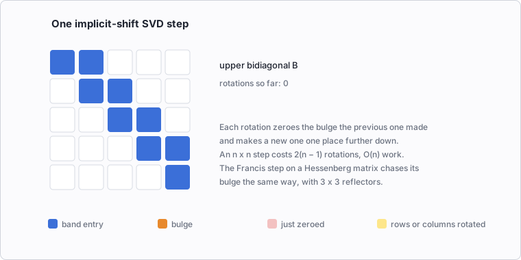
The QR algorithm for eigenvalues and singular values first reduces the matrix to a band: Hessenberg, tridiagonal or bidiagonal. It then repeats a step that keeps the band but makes its off-diagonal entries shrink. The figure shows one Golub–Kahan step on an upper bidiagonal matrix :
- A right rotation on columns 1 and 2 brings in the shift. It creates one nonzero below the band, the bulge.
- A left rotation on rows 1 and 2 zeroes the bulge and creates a new one above the band.
- The rotations alternate, each one zeroing the previous bulge and creating the next one a place further down, until the bulge falls off the corner.
An step costs rotations and work, against for the reduction that came before. Rotations suit this because each one has to remove exactly one entry without disturbing the band.
- Symmetric tridiagonal eigenvalues use the same chase with one rotation
per position. MTL5’s
eigenvalue_symmetricdoes this (include/mtl/operation/eigenvalue_symmetric.hpp). - Nonsymmetric eigenvalues use the Francis double-shift step on a
Hessenberg matrix. Its bulge is , so the chase uses small
reflectors (
include/mtl/detail/francis_qr.hpp). - Singular values in LAPACK (
dbdsqr) use the step in the figure. MTL5’ssvdtakes a different route, one-sided Jacobi (include/mtl/operation/svd.hpp). It applies plane rotations to pairs of columns until they are orthogonal, which is Jacobi’s 1846 method applied to columns.
4. Orthogonality in a narrow format
Section titled “4. Orthogonality in a narrow format”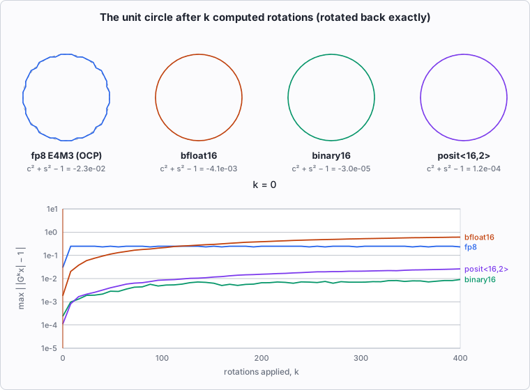
Forty-eight points on the unit circle are rotated 400 times by the same rotation through one radian, with every multiply and add rounded to the format. After each multiple of 8 rotations, the points are rotated back exactly by , so only the error remains: an exact rotation would leave the dashed circle where it is. The chart plots the largest radius error, .
| format | error at | |||
|---|---|---|---|---|
| fp8 E4M3 (OCP, saturating) | ||||
| bfloat16 | ||||
| binary16 | ||||
| posit<16,2> |
Two effects are at work.
- The rounded rotation is not orthogonal. Once and are rounded, , and every application scales the plane by . Applied times, that is a geometric drift of about . bfloat16’s circle shrinks steadily for this reason, so its radius error in the chart keeps growing.
- Every operation rounds. Each multiply and add adds an error of order the unit roundoff. These errors do not share a sign, so they accumulate more slowly, like a random walk. They are what makes the binary16 and posit curves wiggle.
The fp8 points snap to a coarse grid within a few rotations. Its error then stays near 0.25: the format has three fraction bits, and a point on the unit circle cannot move by less than a grid step.
At sixteen bits the ranking depends on the angle. posit<16,2> has 11 fraction bits on , where and lie, against binary16’s 10. For one radian, though, the rounding of and happens to leave posit<16,2> with a larger , and that bias dominates by . At other angles the two swap places, or round to the same and . One extra bit of precision does not guarantee a smaller error in this test.
This is a deliberately harsh test: one rounded rotation applied 400 times, so its bias compounds. A factorization computes a fresh rotation or reflector for every step, from the data in front of it, and the backward error bounds of Higham’s chapter 19 grow only linearly in the number of transformations. Some algorithms do accumulate a long product of transformations explicitly, though: the of an eigensolver, or the of one-sided Jacobi. In a narrow format that product is where to look, by measuring . A square-root Kalman filter instead triangularizes afresh at every step and carries only the triangular factor; how that factor holds up over many steps is a separate question. The mp-numerics studies #13 to #15 make these measurements across formats; the results of #13 are in Givens and Householder across number systems.